Overview
Revisitting the sparse matrix technology - Summary.
Problem Statement
we wish to solve $$ Ax=b $$ with $A$ sparse and symmetric. If $P$ is a permuation matrix, the system of linear equation can be writtem: $$ PAP^TPx=Pb $$ or if $B=PAP^T$, $y=Px$ , and $c=Pb$ $$ By=c $$ where $B$ is the permeated form of $A$ it is also sparse and symmetric. If $A$ is positive definite, $B$ is also positive definite.
The amount of fill-in requred to factorize $B$ depend on $P$. Our goal is to find a convinient $P$ that results in the least possible fill-in after factorisation. $$ argmin_{P}\ ||L||_0\ s.t\ \ \ \ PAP^T = LL^T\ Ax =b\ $$
Motivation of different algorithms
Minimum ordering algorithm
Fill-in are produced during the column elimination.
In order to reduce the number of nonzeros in the i-th column, a natrual idea is to move the column with the fewest nonzeros from the submatrix to the i-th column at each step.
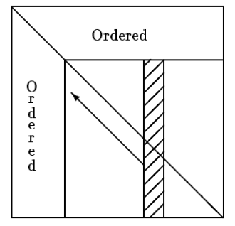
It always prioritizes the nodes with the minimum degree from the unlabelled nodes. One further enhancement method can be referred to the operations on indistinguishable nodes
Reverse Cuthill-McKee (RCM) algorithm
All arithmetic is confined to band and no new zero elements are generated outside of the band.
To minimize the bandwidth of the row associated with z, node z should be ordered as soon as possible after y
The Cuthill-McKee scheme can be regarded as a method that reduces the bandwidth of a matrix via a local minimization of the $\beta_i$’s.
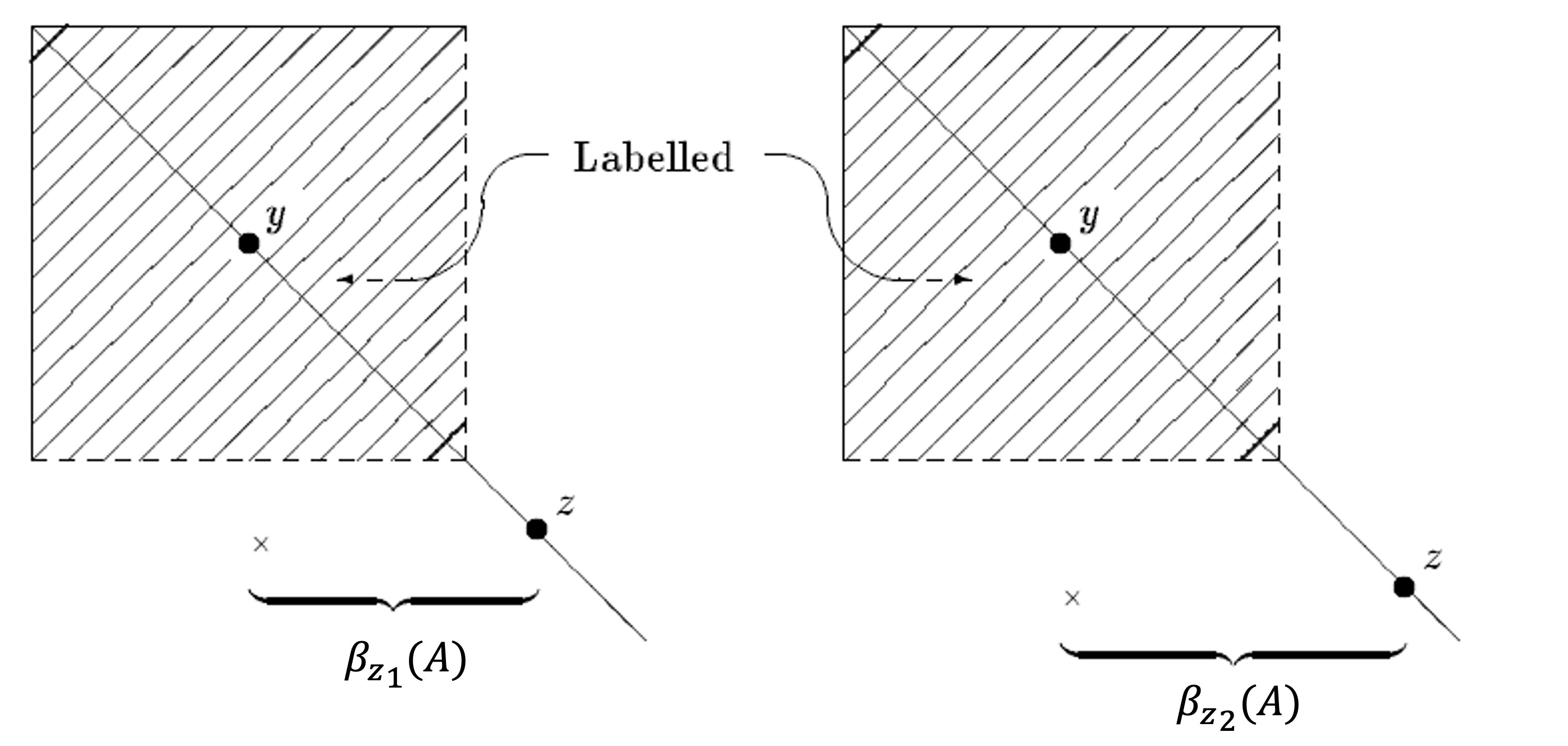
In RCM algorithms: The bandwidth is compressed via a greedy method $$ min\ \beta(A) \rightarrow\ min \sum_i\beta_i(A) $$ The way to find the starting point is also a heuristic method
Nested Dissection Algorithm
Ad: speed, predicitable storage requirement
Our purpose is to preserve as many zero entries as possible. Here we create zero blocks as much as possible by using seperators.

Algorithms
Comparsion
Experiment results
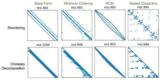
Test case 1: 100x100 mesh matrix
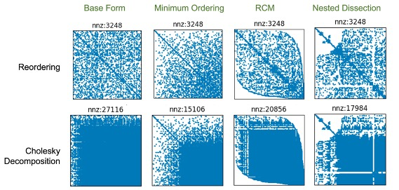
Test case 2: 200x200 random sparse matrix generated by Scipy
Evaluation metrics
It is more or less self-evident that for some classes of problems, one method may be uniformly better than all others, or that the relative merits of the methods in one sector may be entirely different for other classes of problems.
Operations (multiplications and divisions) measures the amount of arithmetic performed
Background $$ Ax=b\ LL^Tx=b\ Ly=b\ L^Tx=y $$
Once computed the factorisation, we must solve the triangular systems via $Ly=b$ and $L^Tx=y$

Alternatively we can compute via the column-wise operation
For a triangular system $Tx=b$, For $i = 1,2,\cdots,n,$ $$ x_i = (b_i-\sum_{k=1}^{i-1}t_{i,k}x_k)/t_{i,i} $$
Terminology
For a given matrix $A$, let $A_{i}$ and $A_{i}$ denotes i-th column and i-th row respectively
Let $\mu(A)$ denotes the number of non-zeros componets of A
The number of operations required to solve for $x$ (Equal or less than the nonzeros of the decomposed components) $$ \sum_i{\mu(T_{*i})|x_i\neq0} $$
Excecution Time: 4 phases:
- Ordering: Finding a good $P$
- Storage allocation
- Factorizing the permutated matrix
- Triangular solution
Storage
Cost(S, T, ….)
Example test data from book
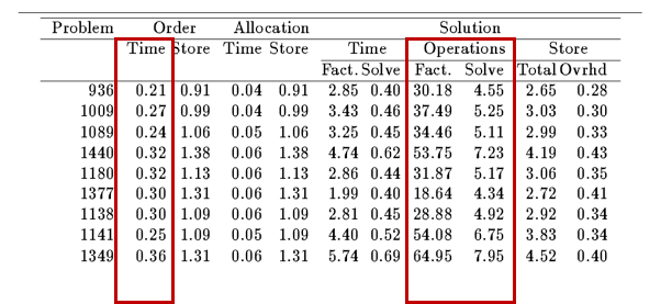
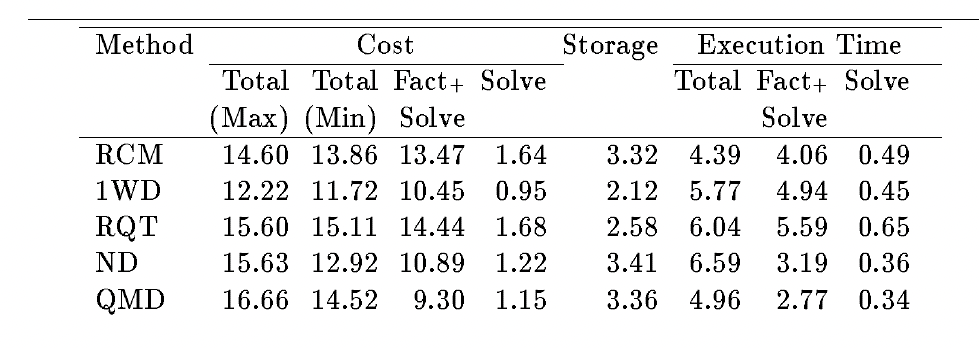
Source: chapter 9 of Computer solution of Sparse Linear system, 1994
There is no simple answer for which algorithms is better, it varies a lot based on the type of the problem, the optimization goal , the size of the problem and the data structure. Nested Dissection tend to be superior to minimum degree for large problems that come from 2D to 3D spatial descretization. Profile reduction method is one of the earlest method which has a direct impact on the memory usage. See more comments from chapter 7.7 of Direct Method for Sparse Linear systems, 2006