Reinforcement Learning Algorithms Summary
1. The connection between Dynamic Programming(DP), Monte-Carlo Method(MC), and Temporal Difference(TD):
1.1 Dynamic Programming
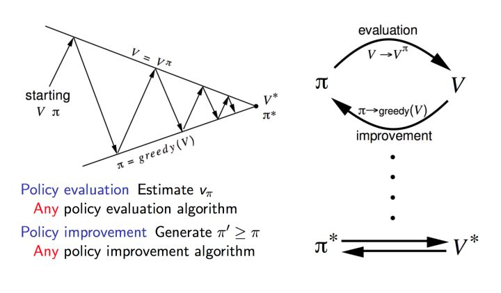
- Taking Policy iteration as an example, the Bellman expectation equation is the key in policy iteration. It is made of two parts: Policy evaluation, and policy improvement.

- In the policy evaluation stage, the method utilizes the Bellman expectation equation to iteratively calculate the state value for the current state until the value is converged.
$$V_{\pi}(s)=\sum_a \pi(a|s)\sum_{s’,r}p(s’,r|s,a)[r+\gamma v_{\pi}(s’)]$$
- In the policy improvement stage:
$$\pi(s) = argmax_a \sum_{s’,r}p(s’,r|s,a)[r+\gamma V(s’)]$$
- Note this is a model-based method since each step needs to know P, the transition probability.
1.2 Monte Carlo Method
- The model is unknown, the value function is estimated by sampling in each episode.
- Update Q value at each end of episodes:
$$Q(s,a) = Q(s,a) +\alpha[\mathbb{E}[R(s,a)]-Q(s,a)]$$
where $\alpha$ is the learning rate, $\mathbb{E}[R(s,a)]$ is the mathematical expectation of $(s,a )$ within one episode.
- Monte Carlo Method uses the practical cumulative rewards as the estimation of the action state value $Q(s,a)$
1.3 Temporal Difference
- Temporal difference utilizes the advantage from both Monte Carlo and Dynamic programming methods.
- Time Difference learns directly from episodes of experience like MD, while experiences are from incomplete episodes by backup methods like DP.
2. Tabular Q-Learning
2.1 Algorithm
Algorithm 1: Tabular Q learning
Initialize Q table
Initialize probability $\epsilon \longleftarrow \epsilon_{max}$
Repeat (for each episode):
Initialize state $s$
Repeat (for each step of the episode)
With probability $\epsilon$ select a random action $a$ otherwise select action $a = \argmax_aQ(s)$
Take action $a$, observe reward $r$, next state $s'$
$Q(s,a)\longleftarrow Q(s,a)+\alpha [r(s,a)+\gamma\max Q(s’)-Q(s,a)]$
$\epsilon \longleftarrow \epsilon * decaying\ factor$
$s\longleftarrow s'$
Until $s$ is terminate
2.2 Temporal Difference
- In Q value update function:
$Q(s,a)\longleftarrow Q(s,a)+\alpha [r(s,a)+\gamma\max Q(s’)-Q(s,a)]$
- where $r(s,a)+\gamma\max Q(s’)$ is the TD target, and $r(s,a)+\gamma\max Q(s’)-Q(s,a)$ is the TD difference.
- By using temporal difference, we do not need to update the value at the end of each episode, while updating at each step by utilizing the Bellman optimality equation (TD target)
3. Deep Q Learning
3.1 Compared with Q learning
- In tabular Q learning, the mapping relation $(s,a)\longrightarrow Q$ are stored as a table. It could lead to a huge waste of time, or even dimensional disaster when searching the related value if $(s,a)$ pairs are too much.
- Deep Neural Network is introduced to replace the Q table in DQN
3.2 Two problems
- Two problems in DQN if only introducing a single neural network:
- Training neural network requires the stochastic samples, while trajectories collected in the environment are highly correlated.
- The target state value is also estimated by the network. It could be unstable since the weight in the network is always updated
- To solve these problems, two mechanisms were introduced in DQN:
- Experience Replay: Randomly choosing a batch of experience$(s,a,s’,r)$ from the experience pool at the end of each episode, breaking the correlation between training samples.
- Fixed Q targets: The second neural network was introduced to specifically estimate the target state value. The update in the target net is relatively slower than the main net, synchronizing the parameters with the main net after every fixed time step.
3.3 Loss functions
- Main Goal
$$Loss = Q^(s,a)-Q(s,a)\Q^(s,a)=R(s,a)+max_{a’}\hat{Q}(s’,a’)$$
3.3 Two networks:
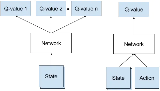
- Policy net $Q$, the input is the state, outputs are state-action values for different possible actions. This is used to choose the optimal action at each step $a_t = \argmax_a Q(s_t,a;\theta)$

- target net $\hat{Q}$, same structure but different task. This network is used for estimating the optimal state-action values by $q=\max_{a’}\hat{Q}(s’,a’;\theta^{-})$
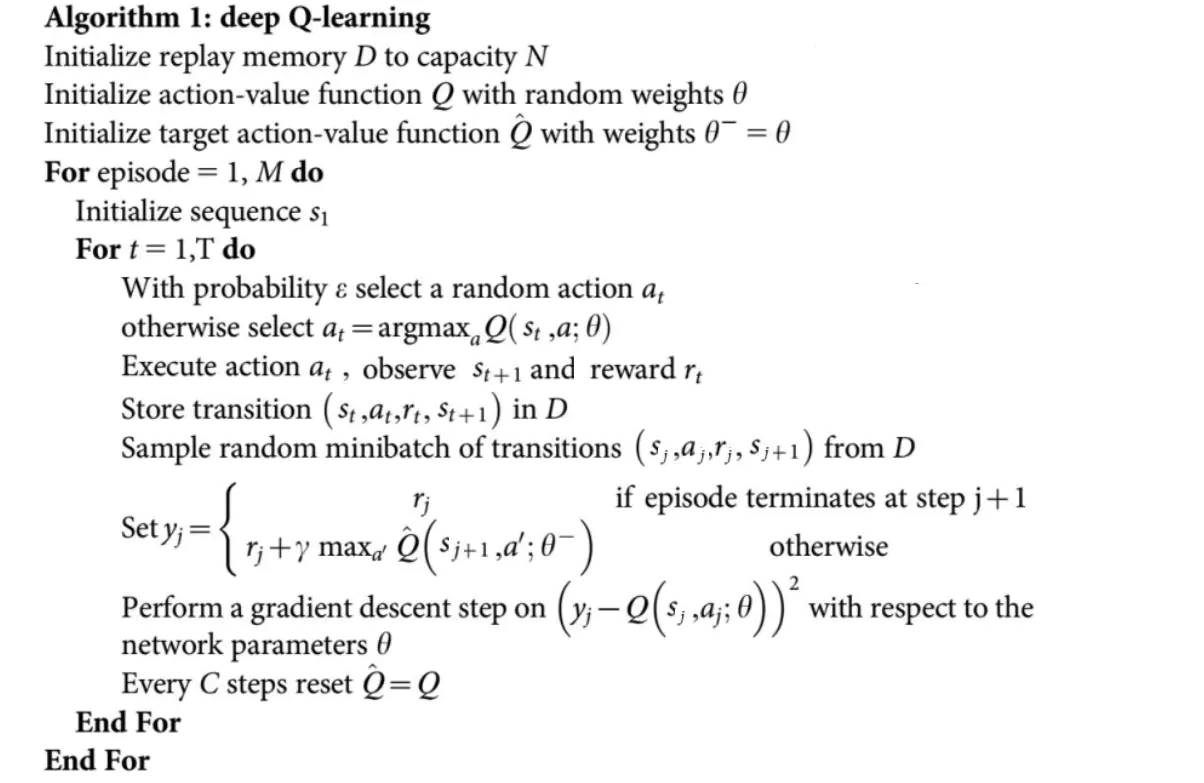
3.4 Algorithm

3.5 Tips in code implementation:
- When estimating the optimal state value, the next state from the step is needed to evaluate the next state value, the next state could be null since the experience were randomly sampled from the pool and the current state could be the last step.

- Note, the next state info in (next_state, reward, done, info) pairs returned by the environment at this time could still be some random float even if the current state is the final state.
3.6 Further improvement
- Double DQN
- Prioritized Replay DQN
- ……
4. Vanilla Policy Gradient
4.1 Policy optimization
- Not like Q learning, policy optimization is on-policy method.
- In reinforcement learning, what we care is about how to choose action under the given state, namely, policy $\pi(a|s)$.
- In Q learning methods, this process is determined by the operation $s\stackrel{\argmax_aQ(s,a)}{\longrightarrow}a$. The policy is indirectly found by repeating this operation with different time steps.
- While in policy optimization, the neural network is trained to directly estimate the policy.
- Another neural network is needed to estimate state value, this is used for calculating the advantage function and guide policy to better update.
4.2 Loss function in policy net
- We want to maximize the expected total return by improving the policy.
$$J(\pi_\theta) = \mathbb{E}{\tau\sim\pi}[R(\tau)]\\theta{k+1} = \theta_k + \nabla_{\theta}J(\pi_\theta)\tag{gradient ascent}$$
- A simplified expression can be obtained after derivation on$\nabla_{\theta}J(\pi_{\theta})$
$$\nabla_{\theta}J(\pi_{\theta}) = \mathbb{E}{\tau\sim\pi{\theta}}[\sum_{t=0}^{T}\nabla_{\theta}\log\pi_{\theta}(s_t|s_t)\hat A_t]$$
- we could utilize Monte-Carlo approximation to calculate the equation, by averaging the trajectory sum at each episode. Hence we got:
$$\nabla_{\theta}J(\pi_{\theta})\approx\hat{g} = \frac{1}{D}\sum_{\tau\in D}\sum_{t=0}^T\nabla_{\theta}\log\pi_{\theta}(a_t|s_t)\hat A_t\tag{1}$$
4.3 Improving the loss function
- $R(\tau)$ in equation (1) is the most basic expression to evaluate how good a policy is. However, in MDPs**, the goodness of action only affects the rewards in the future (after that action), not relating to the rewards before**, and not relating to the whole trajectory. Hence, $R(\tau)$ could be replaced by other improved equations, denoted as $\phi_t$
$$\nabla_{\theta}J(\pi_{\theta}) = \mathbb{E}{\tau\sim\pi{\theta}}[\sum_{t=0}^{T}\nabla_{\theta}\log\pi_{\theta}(s_t|s_t)\phi_t]$$
- Reward-to-go: reward-to-go removes the rewards brought by earlier actions.
$$\nabla_{\theta}J(\pi_{\theta}) = \mathbb{E}{\tau\sim\pi{\theta}}[\sum_{t=0}^{T}\nabla_{\theta}\log\pi_{\theta}(s_t|s_t)\sum_{t’=t}^TR(s_{t’},a_{t’},s_{t’+1})]$$
- Baseline is the method introduced to reduce the variance between different trajectories but not changing the expectation. The most common based line is the on-policy value function $V^{\pi}(s_t)$. Extra: Expected Grad-Log-Prob ( EGLP ) lemma
$$\nabla_{\theta}J(\pi_{\theta}) = \mathbb{E}{\tau\sim\pi{\theta}}[\sum_{t=0}^{T}\nabla_{\theta}\log\pi_{\theta}(s_t|s_t)[\sum_{t’=t}^{T}R(s_{t’}, a_{t’}, s_{t’+1})-V^{\pi}(s_t)]]$$
- Advantage function: advantage function is defined as discounted rewards - baseline estimated, in VPG, the advantage is:
$$A(s,a)=Q(s,a)-V(s,a)=\phi_t(s,a)$$
- Adding all together: The loss function in VPG is:
$$L(\theta) =\mathbb{E}t[\log\pi{\theta}(a_t|st)\hat{A}_t]$$
4.4 Loss function in target net
- Another network is needed to estimate the value function since it was used in advantage function.
- The loss is calculated by mean square error and the net is fitted by gradient descent.
$$target\ value\ loss=MSE(V^{\pi}(s_t), \hat{R}_t)$$
4.5 Algorithm
4.5 Generalize Advantage Estimate (GAE)
$$\hat{A_t}^{GAE(\gamma,\lambda)} = \sum_{l-1}^{\infty}(\gamma\lambda)^l\delta_{t+1}^V\=\sum_{l=1}^{\infty}(r_t + \gamma V(s_t +\gamma V(s_t +l+1)-V(s_{t+l})))$$
5. Proximal Policy Optimization
5.1 Drawbacks of basic VPG:
- Training data sets are collected by interacting with the environment, and data distribution over states and rewards are constantly changing, making the prediction unstable.
- Very high sensitivity of hyper parameters.
5.2 Loss function
$$\mathbb{E}t[L_t^{CLIP}(\theta)-c_1L_t^{VF}(\theta)+c_2S[\pi{\theta}(s_t)]]\tag{1}$$
- where the first part of equation 1 is the central objective function of the policy net:
$$L^{CLIP}(\theta) = \mathbb{E_t}[\min(\frac{\pi_\theta(a_t|s_t)}{\pi_{\theta_{old}}(a_t|s_t)}\hat{A_t},\ clip(\frac{\pi_\theta(a_t|s_t)}{\pi_{\theta_{old}}(a_t|s_t)},1-\epsilon,1+\epsilon)\hat{A_t}]\tag{2}$$
- The first part is the normal policy gradient objective which pushes the policy towards actions that yield a high positive advantage over the based line
- The second is nothing but new but adding a clipping operation, making the probability of actions change under two conditions. (The advantage function is noisy and we do not want to destroy our policy based on on a single estimate!!):
- If the advantage is positive (action is good), it clips the objective function if $\frac{\pi_\theta(a_t|s_t)}{\pi_{\theta_{old}}(a_t|s_t)}$ is too large since we don’t want to overdo the action too much.
- If the advantage is negative (action is bad), it flattens the objective function if $\frac{\pi_\theta(a_t|s_t)}{\pi_{\theta_{old}}(a_t|s_t)}$ is near zero since we also don’t want to reduce these action probability to zero
- min operator plays its role when the $\frac{\pi_\theta(a_t|s_t)}{\pi_{\theta_{old}}(a_t|s_t)}$is big but making the policy worse, the min operator will choose the normal policy objective function instead of clipped version since this is the only region that the normal version is lower than the clipped version
- The second part of equation 1 is the loss function of the target net, which is basically in charge of updating the baseline network ($\hat{A}_t$)
$$L_t^{VF}(\theta)=\mathbb{E_t}[\hat{R}_t - V_t(s_t)] \tag{3}$$

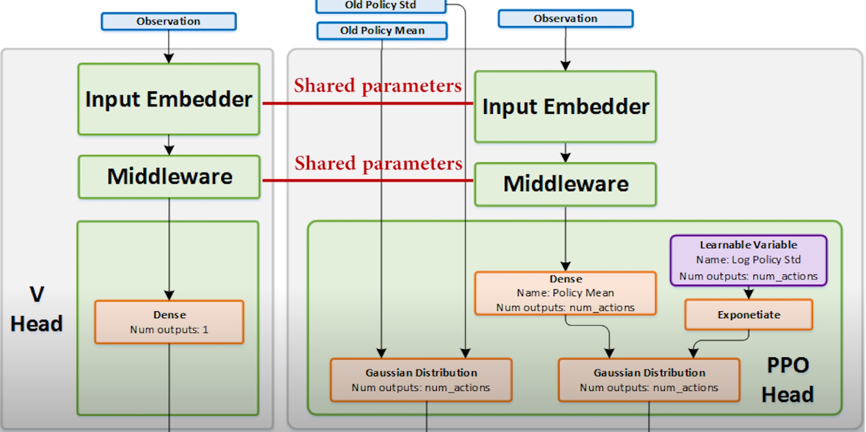
The value estimation network shares a large portion of parameters with the policy estimate network (similar feature pipelines), hence we put losses into one equation and the
The third part of the equation is the entropy bonus term which ensures the agent does enough exploration during train
third part of equation 1 : entropy bonus
to transmit one bit of information means to reduce the recipient’s uncertainty by a factor of 2
- suppose $p_i$ is the probability of event $p$:
$$Entropy:H(p)=p_1\times\log_2 \frac{1}{p_1} +p_2\times\log_2 \frac{1}{p_2}+p_3\times\log_2 \frac{1}{p_3}+……\=-\sum_i p_i\log_2(p_i)$$
- It measures average amount of information that you get from one sample drawn from a given probability distribution. It tells you how unpredictable that probability distribution is.
$$L^{VF}(\phi) = \frac{1}{N}\sum$$