Overview
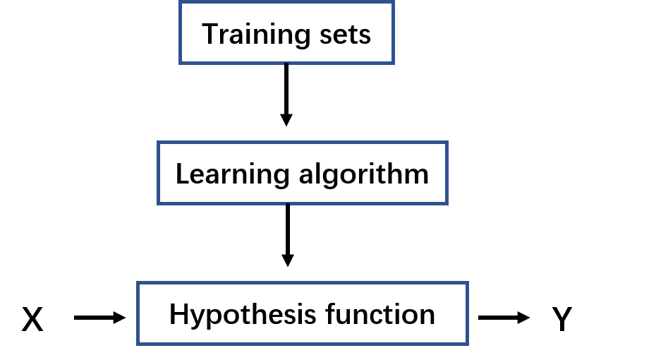
In the linear regression prediction, we want to find a hypothesis function to predict the future outcome. The method in supervised learning is by using loads of training data sets and a learning algorithm to let the result of the hypothesis function close to the real value as possible as we can.
The process can loosely be represented by the following flowchart:

Training sets are the data we got from the previous experience, which contains the input feature (X), and the training example(Y). It can be represented by $$ (x^{(i)},y^{(i)}) $$ where *i *is the index of the training sets
The hypothesis or saying, prediction function is a linear regression function: $$ h_{\theta}(x)=\theta_0 + \theta_{1}x $$ Where $\theta_0$ and $\theta_1$ are the parameters that we look for to minimize the cost function.
Cost Functiom
In order to let the result of the hypothesis function as close to the real result as possible, we need to find the specific $\theta_0$and $\theta_1$, and we have to try different values for these two variables. To normalize and evaluate output results with different parameter values, we use the cost function: $$ J(\theta_0, \theta_1)=\frac{1}{2m}\sum^m_{i=1}[h_\theta (x^i)-y^{(i)}]^2 $$ Where
- i is the index of the data sets
- mis the number of data sets
- *$h_\theta(x^{(i)})$*is the hypothesis output
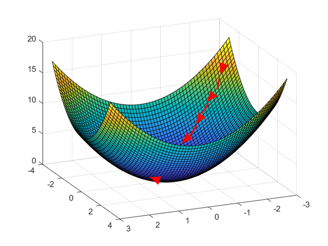
- $y^(i)$ is the real example value Since it has a constant scalar output for each sets of training data, $J(\theta_0, \theta_1)$ can be seen as a scalar field. (always a convex bowl-shape field)

Summary
So far, we got hypothesis function: $$ h_\theta(x)=\theta_0 +\theta_1 x $$ With parameters: $$ \theta_0, \theta_1 $$ Cost function is: $$ J(\theta_0,\theta_1)=\frac{1}{2m}\sum^m_{i=1}[h_\theta(x^{(i)})-y^{(i)}]^2 $$ Goal is: $$ minimize\ J(\theta_0, \theta_1) $$
Gradient Descent Algorithm
basic idea

- start with a point
- keep finding the steepest direction of the current position and moving down a small step
- until end up at a minimum.
formula
$$ \theta_j := \theta_j -\alpha \frac{\partial}{\partial \theta_j}J(\theta_0, \theta_1) $$ $$ (for\ j=0\ and\ j=1) $$ Note: The new value assignment for $\theta_0$ and $\theta_1$ have to be updated simultaneously.
Where
- :=” is the assignment operator, on the right side, $\theta_j$ is the current parameter; on the left side, $\theta_j$ is the next new value. The minus operation will be repeated until convergence.
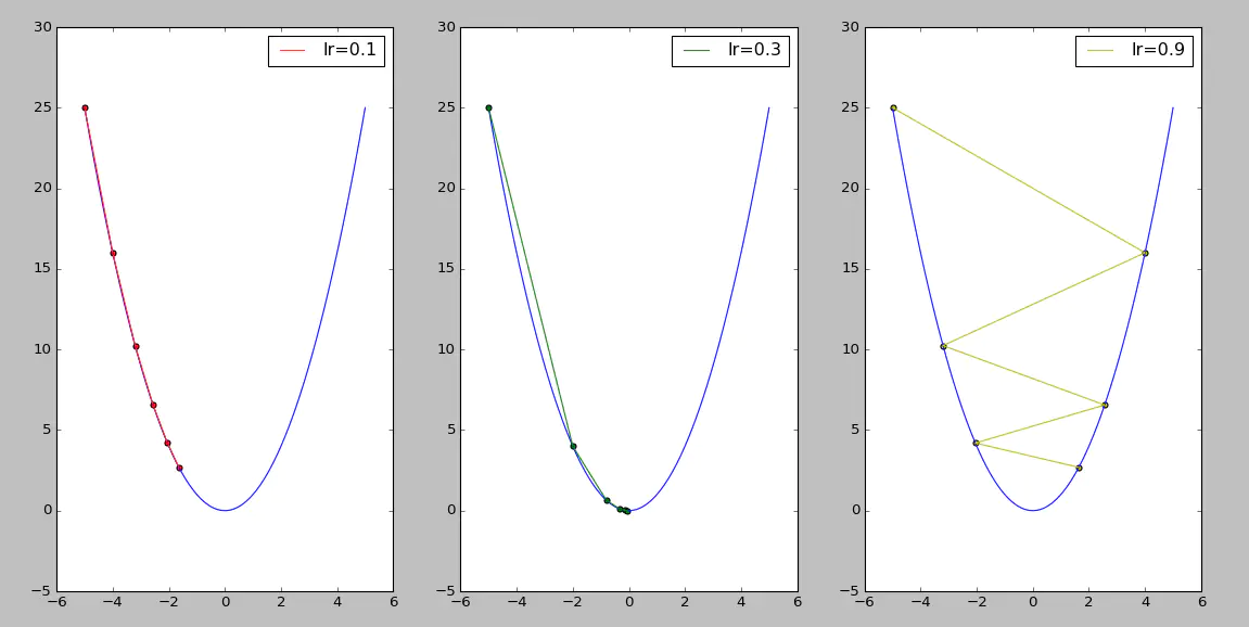
- $\alpha$ is the learning rate, or saying how long your every down step distance is,
- $\frac{\alpha}{\alpha \theta_j}J(\theta_0, \theta_1)$ is nothing but the partial derivative of the cost function.
Conclusion derive
$$ \frac{\partial}{\partial \alpha_j}J(\theta_0, \theta_1) $$ $$ =\frac{\partial}{\partial \theta_j}[\frac{1}{2m}\sum^m_{i=1}[h_\theta(x^{(i)})-y^{(i)}]^2] $$ $$ =\frac{1}{2m}\frac{\partial}{\partial\theta_j}\sum^m_{i=1}[\theta_0+\theta_1x^{(i)}-y^{(i)}]^2 $$ When j = 0: $$ =\frac{1}{2m}\frac{\partial}{\partial\theta_0}\sum^m_{i=1}[\theta_0+\theta_1x^{(i)}-y^{(i)}]^2 $$ $$ =\frac{2}{2m}\sum^m_{i=1}[\theta_0 + \theta_1 x^{(i)}-y^{(i)}] $$ $$ =\frac{1}{m}\sum^m_{i=1}[h_\theta(x^{(i)})-y^{(i)}] $$
When j =1: $$ =\frac{1}{2m}\frac{\partial}{\partial \theta_1}\sum^m_{i=1}[\theta_0+\theta_1x^{(i)}-y^{(i)}]^2 $$
$$ =\frac{2}{2m}\sum^m_{i=1}[\theta_0+\theta_1x^{(i)}-y^{(i)}]\cdot x^{(i)} $$
$$ =\frac{1}{m}\sum^m_{i=1}[h_\theta(x^{(i)})-y^{(i)}]\cdot x^{(i)} $$
Take the derived conclusions back to the algorithm, we now got the simplified algorithm to find a particular pair of ($\theta_0$, $\theta_1$) for our hypothesis function: $$ \theta_0 :=\theta_0 -\alpha\frac{1}{m}\sum^m_{i=1}[h_\theta(x^{(i)})-y^{(i)}] $$
$$ \theta_1 :=\theta_1-\alpha\frac{1}{m}\sum^m_{i=1}[h_\theta(x^{(i)}) - y^{(i)}\cdot x^{(i)} $$
Note: update $\theta_0$and$\theta_1$ simultaneously.
Some thoughts and questions
Q: Since the cost function is a convex, scalar field in linear regression, and the goal is to find the minimum, why don’t we just let the gradient = 0 to find the minimum stationary point of this field?
A:
- Not all functions can find the point where the value of zero that obtained according to the derivative.
- Sometimes, the value of the derivative at each point can be obtained, but the direct solution of the equation cannot be solved.
- Or when the amount of data is large, the inverse of the matrix is required, which is very resource-consuming.
- n general, it is more effective than linear algebra solutions for mega-problems. When you have thousands of variables (such as machine learning), this becomes more important as the dimensions increase.
- we need to teach the computer how to calculate the root of the derivative of function.
Q: How to choose the learning rate $\alpha$ in the algorithm? How does it affect?
A:
- Firstly, gradient descent can converge to a local minimum, with the learning rate fixed. As we approach a local minimum, gradient descent will automatically take smaller steps since the gradient is decreased at the same time
- If the rate is too small, gradient descent can be slow. If the rate is too large, gradient descent can overshoot the minimum.

- Momentum
Momentum is a physic theory that can describe that as the iterative process continues, the learning rate is appropriately reduced in order to reach the extreme point more smoothly. It shows that the running state of the moment before has an impact on the moment. In physics, it means the cumulative effect of expressive force on time.
In the previous equation, the decrement of each time (saying v) is represented by: $$ v=-\alpha\cdot\frac{\partial}{\theta_j}J(\theta_0,\theta_1) $$ Consider the decrement v as the current gradient descent amount $-\alpha\cdot\frac{\partial}{\theta_j}J(\theta_0,\theta_1)$ and the last update amount v multiplied by a factor momentum between [0, 1]: $$ v=-\alpha\cdot\frac{\partial}{\theta_j}J(\theta_0,\theta_1) +v\cdot momentum $$ When the direction of the current decrement is the same as the direction of the previous decrement. The previous decrement will play an acceleration role in the current search.
When the direction of the current decrement is opposite from the direction of the previous decrement. The previous decrement will play a deceleration role in the current search.
Reference: https://www.jianshu.com/p/58b3fe300ecb